It’s a Thursday morning, and the VP of Sales is staring at a spreadsheet. One number — 10.1% — is about to end someone’s career. He doesn’t know it yet, but he’s about to make a decision that mathematics would call premature.

I would call this problem “Promote or Fire”, or “Let’s Fire Grandma”.

Here we’re looking at our sales department’s results, and questions are arising about our new manager, Drennan:

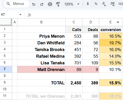
Matt Drennan joined the team two and a half months ago. He came from a smaller company, interviewed well, and his first few weeks were promising — he learned the product fast, clients liked him on the phone. His probation target was set at “16 deals per 100 calls”. Reason? Because historically, our VP of Sales observed a call-to-deal conversion rate of 16.1%.

Now, with 89 calls behind him and only 9 deals to show for it, his conversion sits at 10.1%.

“Fire him,” the VP of Sales decides.

Here’s the question: is this decision justified? Has enough time passed (enough data accumulated) to make this call? Has the “bad luck” factor been accounted for? Could it be that Drennan is simply performing no worse than the other managers, actually converting at around the required 16%, but consistently running into clients’ force majeure events (5 clients “dropped off”), a “rough patch” in his personal life, and an unfortunately positioned Moon in the third house of Taurus?

Rolling the Dice

Before we get to the spreadsheet formula that will settle this, let me take you on a brief detour.

In 1913, at the Monte Carlo Casino, the roulette ball landed on black twenty-six times in a row. Gamblers lost millions betting against the streak, convinced that red was “due.” They were wrong — not because the wheel was rigged, but because they could not intuitively grasp what randomness actually looks like. Streaks happen. Cold spells happen. And sometimes a perfectly good sales manager just has a bad quarter.

This is the same trap the VP of Sales is walking into.

Recalling the coin flip example, let’s switch things up this time and roll a 6-sided die. The probability of rolling a “1” is 1/6, or roughly 16.7%.

The expected value for 89 rolls of a die is 89 × 1/6 = 14.8 “ones” (and the same number of “twos,” “threes,” and so on), but obviously you could get not just 14–15, but also 12, 17, or even 20. Getting none at all, however, is virtually impossible (though, theoretically, the probability isn’t zero).

Drennan’s work can be thought of as rolling a die, where the desired outcome — a “one” (a deal) — comes up roughly every sixth roll. Roughly, because the historically observed conversion rate (excluding Drennan’s results) is 380 deals out of 2,361 calls, or 380/2,361 = 16.1%. The expected value from his 89 “rolls” (calls) is 89 × 0.161 = 14.3 “ones” (deals), but intuitively, we understand there could be slightly more or slightly fewer.

If we calculate (we’ll learn how shortly) the exact probabilities of “landing” a specific number of deals in 89 calls and plot them on a graph, the most likely outcome (the “expected value”) of 14 deals will be in the center, with the remaining possible outcomes (13 and 15 deals, 12 and 16 deals, etc.) becoming progressively less likely each time, giving the graph its bell shape:

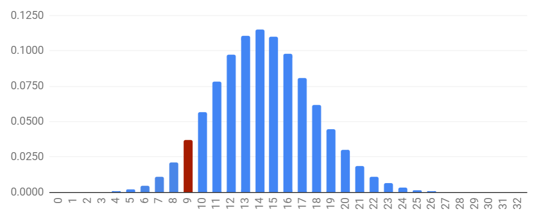
We can’t say that 9 deals is entirely improbable — the bar is visible, if modest, with a probability of 0.037. That is, it happens in 1 out of 27 cases — which may be unlikely, but not extremely unlikely.

All that’s left is to figure out how we arrived at “1 in 27,” and how this connects to difficult, “staff”, decisions in a sales department.

Calculating the Binomial Distribution

Both Excel and Google Sheets have a built-in binomial distribution function. It’s exactly what will give us the answer to whether it’s time to fire the unlucky Drennan.

In the cell next to his 10.1% conversion rate, we calculate the function:

=BINOM.DIST(D7,C7,$E$11,1)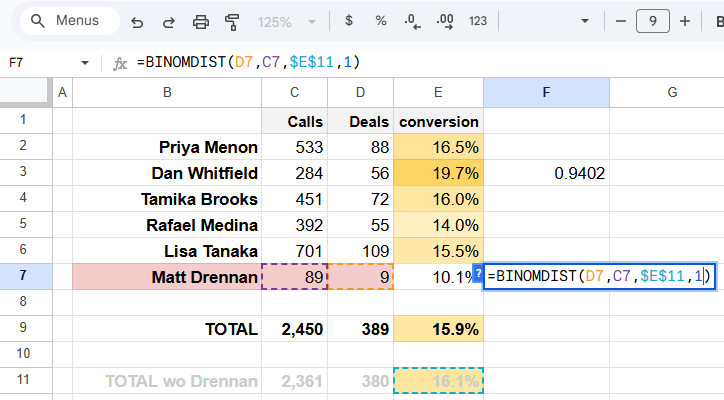

In this function, we specify, in order: the number of successes (deals), the number of trials (calls), and the probability of success (the 16.1% conversion rate). The last, 4th parameter, we set to “1.”

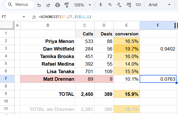
What is this 0.0763 we got? 0.0763 is the probability of getting no more than 9 deals out of 89 calls given a deal probability of 16.1%. In other words, it’s the probability of getting anywhere from 0 to 9 deals inclusive with these parameters. Conversely, 1 − 0.0763 = 0.9237 is the probability of getting 10 or more deals.

(By the way, if you change the 4th parameter to “0,” you get the probability of getting exactly 9 deals.)

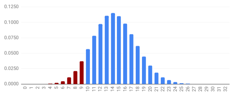
You could say that, taking the sum of all bars on the graph as 1, the sum of bars “0” through “9” equals 0.0763, or 7.63%. As you can see, it’s far more likely to land in the blue portion of the bell curve than in the red one (92.37% vs. 7.63%).

Conclusion: the probability that Drennan, while actually converting at 16.1%, would randomly (remember the possibility of a “rough patch”?) end up with no more than 9 deals out of 89 calls is 7.63%.

Conversely, there’s a 92.37% probability that he would have gotten 10 or more deals. Roughly speaking, there’s a 7.63% chance he was simply unlucky, and a 92.37% chance that bad luck alone doesn’t explain it, and he is most likely converting at a rate below 16.1%.

Therefore, if a 90% confidence level is enough for the VP of Sales, then Drennan can be let go at the end of his probation — the manager is, indeed, not meeting his target. If, however, a 95% confidence level is required, the data is not yet sufficient, and it would be advisable to observe a bit longer.

So what confidence level should we choose? There is no right answer here.

If we set it too low, we risk accidentally firing good managers, but we won’t lose deals by continuing to work with bad ones.

If we set it too high, we’ll have to accumulate data for too long before making a mathematically justified decision to fire a bad manager, but the probability of accidentally firing a good one will be lower. In my opinion, a 90% level is optimal for this case. Drennan can be fired.

Wait, What About Whitfield’s 19.7%?

Indeed, if there are “bad” managers for whom there’s a 92.37% probability that their conversion is below the required 16.1%, then logically, there can also be “good” ones.

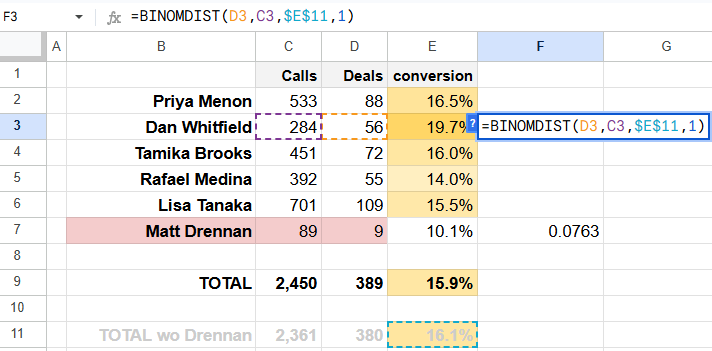
Dan Whitfield is the quiet opposite of Drennan. He’s been with the company for six months, never makes a fuss, never asks for a raise. He just dials, talks, and closes. Over that time he put up 56 deals on 284 calls — a 19.7% conversion rate — compared to the projected 0.161 × 284 = 46 deals. Could he have been lucky this whole time? Could it be that, while actually performing like everyone else at a 16.1% conversion rate, he randomly ended up with more deals than the VP of Sales projected?

The binomial distribution function returns 0.9563 — meaning that with a 95.63% probability, working like everyone else, he would have gotten no more than 56 deals... but he didn’t get more than 56 deals... He got exactly 56!

Let’s simply refine the function by recalculating it for 56 − 1 = 55 deals:

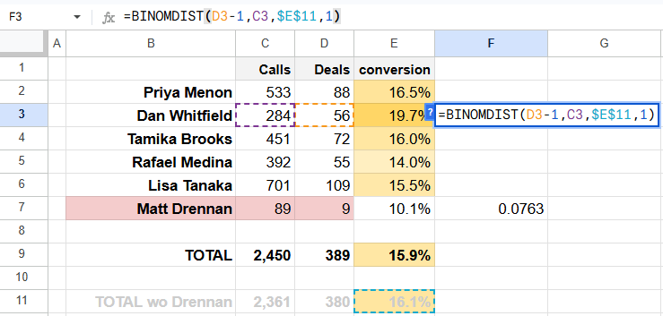
For 55 deals, the result is 0.9402. That is, with a 94.02% probability, Whitfield (working at a 16.1% conversion rate) would have gotten no more than 55 deals. This means the probability of getting more than 55 deals is the remaining 5.98%! It turns out our Whitfield landed in a sliver of his own bell curve — just on the opposite end — and the probability of landing there is only about 6%.

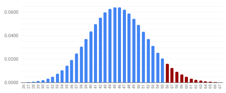
The VP of Sales has already decided that before making staffing decisions, he wants to be at least 90% confident in the results. And in Whitfield’s results, he’s 94.02% confident! That leaves only 5.98% for the possibility that Whitfield was simply lucky.

So either he got lucky, even though he actually performs like everyone else (at a 16.1% conversion rate) and doesn’t deserve a higher salary, or he truly converts at a rate above 16.1% and it would be fair to reward him.

6% clearly loses to 94%, so Whitfield gets the promotion.