I’ve been happily using a more informative way to visualize conversion rates for a while now, by adding confidence interval bounds to my charts.

Sales office conversion rates

Say we’re evaluating the performance of regional sales offices. By performance we mean the ratio of closed deals to incoming leads (lead-to-sale conversion, or simply “conversion”). For example, if the “Midtown” office closed 19 deals out of 33 leads in a quarter, we consider their performance to be 19/33 = 57.6%.

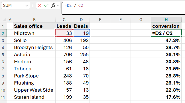
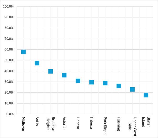
Clearly, some offices outperform others: conversion rates range from 57.6% down to 17.6%. It is also apparent that the number of leads varies widely across offices: from 33 leads in “Midtown” to 706 leads in “Astoria.”

Most people would stop here, but there is a straightforward way to use the concept of a “confidence interval” or “standard deviation (SD)” to reveal something that isn’t immediately obvious.

Estimating sample size and SD

Because the number of leads differs dramatically across offices (“Midtown” and “Astoria” differ by a factor of nearly 22), our confidence in the calculated conversion rate will not be uniform. For “Astoria,” the 36.1% figure is based on a sample of 706 leads and can be considered quite reliable. For “Midtown,” the 57.6% result comes from a small sample of just 33 leads, so there is no guarantee that, given their own 706 leads over time, they would sustain the same conversion rate.

Naturally, we need to estimate the confidence interval for each sales office based on the number of leads — that is, the sample size.

Here is the familiar formula for the standard deviation (SD), or σ:

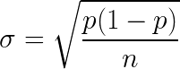
where p is the conversion rate and n is the number of leads.

We compute it in column E:

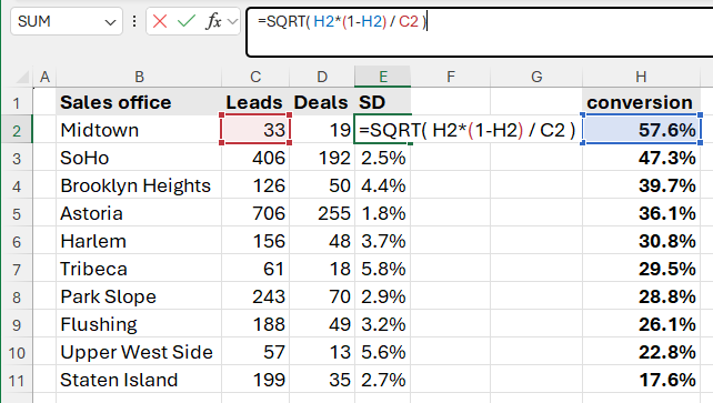
The resulting standard deviation shows the margin of error in the conversion estimate. As expected, it is larger where the sample is smaller. The less data we have, the less reliable the calculated result, and the less confident we can be in our assessment of the corresponding office’s performance.

Computing the bounds of a 90% confidence interval

Let us extend our table with the lower and upper bounds of a 90% confidence interval. In other words, we estimate the range of conversion rates for each office such that there is a 90% probability the true conversion rate falls within that range.

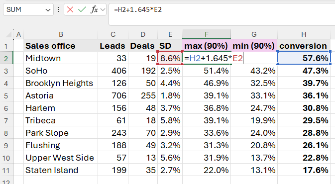
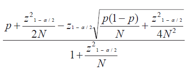
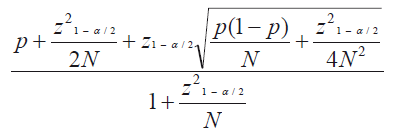
Knowing that the bounds of a 90% confidence interval lie at ±1.645 SD, we subtract and add 1.645 SD to obtain the lower and upper bounds, respectively. For “Astoria,” this tells us that the true conversion rate lies between 33.1% and 39.1%. (One time out of ten it may still fall outside our interval, but nine times out of ten our estimate holds.)

Enhancing the chart with “candlesticks”

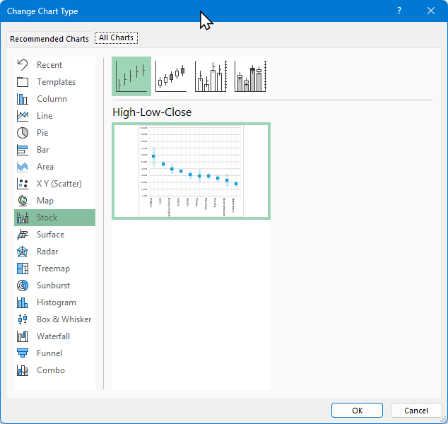
In Excel 2013 we can use a “stock chart,” substituting the upper and lower confidence interval bounds for the high and low prices, and the conversion rate calculated earlier for the close price:

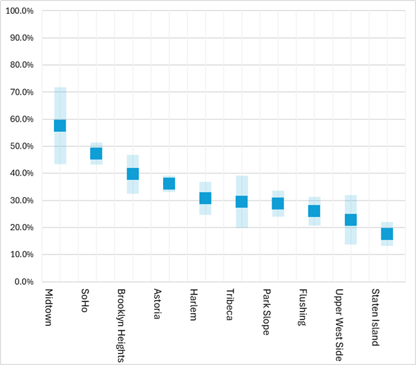
The enhanced chart does not change the conclusions we drew at the outset. However, it subtly reminds an observant manager that the reported conversion rates are not final — and are especially “not final” where the confidence bounds are wider.

“Midtown” appears to have outperformed “SoHo”, but while “SoHo” strong result is reliable thanks to its narrow interval, the result for “Midtown” is highly approximate. Definitive conclusions can therefore only be drawn for some of the offices; for the rest, more data is needed, and until then their rankings should be considered preliminary — or, as noted above, not final.

You listen to 10 random call center calls. In 4 of them, the operator never asks the client where they heard about you from. So now you have a number: 40% of calls are missing the advertising source. That’s an issue. You bring it to your manager, maybe flag it in a report.

But here’s the thing. Is it really 40%?

The trouble with small samples

10 calls is not a lot. You picked them at random, and randomness is fickle. The true failure rate could be 20%. It could be 60%. You just don’t know — and the small sample is the reason.

There is, of course, a standard way to express this uncertainty. You calculate the SD of the binomial distribution:

You get SD = 15.49%. Then you build a 90% confidence interval: 40%±1.645 SD, which gives you a range from 14.52% to 65.48%.

That’s a huge spread. But at least now you’re honest about it: with 90% probability, the true failure rate lies somewhere in that range.

The 40% figure is just your best guess, not a fact.

So far, so good.

Except there’s a catch.

When the standard method breaks down

The ±1.645 SD approach works well enough — until it doesn’t. When your sample is small or your proportion is extreme (very close to 0% or 100%), the formula starts to wobble. There’s a simple rule of thumb: if np < 10, you’re in trouble. In our case, np = 4. We’re in trouble.

Think of it this way. If “tails” came up fewer than 10 times, either you haven’t flipped the coin enough, or you’re dealing with a biased coin that rarely lands on tails. Either way, the standard formula isn’t built for this.

Many statisticians consider the Wilson method to be the most reliable approach for estimating confidence intervals for proportions <...>. This method not only handles very small and very large proportions, but also works well with small sample sizes.

The method was proposed in 1927. It has been around for nearly a century. And yet most analysts still reach for ±1.645 SD by default.

The Wilson method

The lower and upper bounds of the confidence interval p = 1–α/2 are computed using the following formulas:

Formulas for the lower and upper bounds, respectively.

where p is the observed proportion, N is the number of trials, and z is the z-score (e. g., 1.960 for a 95% confidence interval, or 1.645 for 90%).

Back to the call center

Let’s revisit our 10 calls. The standard method gave us a confidence interval from 14.52% to 65.48%. Now let’s apply Wilson.

The bounds tighten: with 90% probability, the true failure rate lies between 19.42% and 64.84%. The effective SD drops to 13.80%.

The difference may look subtle, but notice what happened at the lower end: it shifted from 14.52% to 19.42%. That’s not a rounding error. In a real business decision — say, whether to retrain your call center team — that shift matters.

And this is the point. When your data is scarce, every percentage point of precision counts. The Wilson score interval doesn’t give you more data. It just makes better use of the data you already have.

Calculator in Google Sheets (menu “File” → “Make a copy”).

See also:

Online calculator for a 95% confidence interval
Calculator on WolframAlpha.com
Binomial confidence intervals and contingency tests (pp. 4–5)
https://influentialpoints.com/Training/confidence_intervals_of_proportions.htm#wils
Wilson score interval on Wikipedia

Here’s a puzzle. Two employees get rated by their clients on a 1-to-5 scale. Their average scores are identical:

Johnson — 5, 5, 5, 5, 5, 2, 2, 2, 2, 2. Average = 3.50.
Miller — 4, 4, 3, 3. Average = 3.50.

A tie. Except — it doesn’t feel like a tie, does it? Johnson has ten ratings, all over the map. Miller has four, tightly clustered. Shouldn’t that matter?

It does. And a fascinating article on EvanMiller.org, “Ranking Items With Star Ratings,” shows exactly how. (Judging by the author’s tone, the whole business of ranking things by ratings is far thornier than it looks, and he keeps coming back to it.)

The core problem is simple: a plain average ignores how many votes went into it. A 4.8 rating from 300 reviews is not the same as a 4.8 from 6 reviews. The first one you can trust. The second one — who knows.

The solution comes from Bayesian statistics (whatever that might mean in this context exactly), et voilà:

Johnson — 2.72
Miller — 2.63

Somehow, either the tighter spread of Miller’s scores (SD of 0.58 vs. 1.58), or the smaller number of ratings (4 vs. 10), or both together refined the average, giving Miller the edge by a few hundredths. The tie is broken.

The formula behind the advanced rating

Brace yourself. It’s gonna sting a little.

We assume there are K possible ratings, indexed by k, where each rating is worth s_k points (“1” = 1 point, “2” = 2 points, and so on). Given N total ratings for each item, with n_k ratings for each k, we can compute the item’s score using the following formula:

Where z_α/2 is the 1−α/2 quantile of the normal distribution. The resulting score is the lower bound of a normal approximation to the Bayesian confidence interval for the average rating. Setting, say, α=0.10 (z=1.65), the score S means that in 95% of cases, the item’s true average rating will be above S.

In plain English: the “advanced” calculation gives you a conservative estimate of what the average rating would converge to if you had more data. And — as we saw with Johnson and Miller — it lets you rank items even when their plain averages are identical.

The advanced rating in action

I took 2,000 ratings on a 1-to-5 scale across a set of regional sales offices and computed both the plain average and the “advanced” score for each one.

Average 1.0 — plain average rating; Average 2.0 — advanced average rating.

Flushing dropped from 2nd to 4th place. The likely reason: its 66 ratings don’t inspire enough confidence that the average is truly that high. In 90% of scenarios, its predicted rating is no better than 4.55 — roughly 4th place territory.

Tribeca, on the other hand, was formally 13th. But thanks to a solid base of 249 ratings, the model predicts — with 90% confidence — an average of at least 4.4, which bumps it up to 10th.

My impression is that the formula works most convincingly for short rating scales, like the 1-to-5 used here.

In any case, here is a Google Sheets workbook — it should handle rating scales up to 100, import up to 10,000 rows of individual ratings, and lets you adjust the confidence level (90% in our example).

See also

https://www.evanmiller.org/ranking-items-with-star-ratings.html

Advanced rating calculator in Google Sheets