
You listen to 10 random call center calls. In 4 of them, the operator never asks the client where they heard about you from. So now you have a number: 40% of calls are missing the advertising source. That’s an issue. You bring it to your manager, maybe flag it in a report.
But here’s the thing. Is it really 40%?
The trouble with small samples
10 calls is not a lot. You picked them at random, and randomness is fickle. The true failure rate could be 20%. It could be 60%. You just don’t know — and the small sample is the reason.
There is, of course, a standard way to express this uncertainty. You calculate the SD of the binomial distribution:
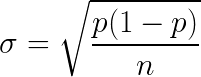
You get SD = 15.49%. Then you build a 90% confidence interval: 40%±1.645 SD, which gives you a range from 14.52% to 65.48%.
That’s a huge spread. But at least now you’re honest about it: with 90% probability, the true failure rate lies somewhere in that range.
The 40% figure is just your best guess, not a fact.
So far, so good.
Except there’s a catch.
When the standard method breaks down
The ±1.645 SD approach works well enough — until it doesn’t. When your sample is small or your proportion is extreme (very close to 0% or 100%), the formula starts to wobble. There’s a simple rule of thumb: if np < 10, you’re in trouble. In our case, np = 4. We’re in trouble.
Think of it this way. If “tails” came up fewer than 10 times, either you haven’t flipped the coin enough, or you’re dealing with a biased coin that rarely lands on tails. Either way, the standard formula isn’t built for this.
Many statisticians consider the Wilson method to be the most reliable approach for estimating confidence intervals for proportions <...>. This method not only handles very small and very large proportions, but also works well with small sample sizes.
The method was proposed in 1927. It has been around for nearly a century. And yet most analysts still reach for ±1.645 SD by default.
The Wilson method
The lower and upper bounds of the confidence interval p = 1–α/2 are computed using the following formulas:
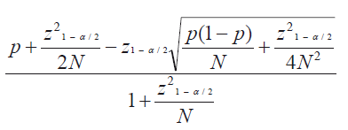
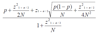
where p is the observed proportion, N is the number of trials, and z is the z-score (e. g., 1.960 for a 95% confidence interval, or 1.645 for 90%).
Back to the call center
Let’s revisit our 10 calls. The standard method gave us a confidence interval from 14.52% to 65.48%. Now let’s apply Wilson.
The bounds tighten: with 90% probability, the true failure rate lies between 19.42% and 64.84%. The effective SD drops to 13.80%.
The difference may look subtle, but notice what happened at the lower end: it shifted from 14.52% to 19.42%. That’s not a rounding error. In a real business decision — say, whether to retrain your call center team — that shift matters.
And this is the point. When your data is scarce, every percentage point of precision counts. The Wilson score interval doesn’t give you more data. It just makes better use of the data you already have.
Calculator in Google Sheets (menu “File” → “Make a copy”).
See also:
Online calculator for a 95% confidence interval
Calculator on WolframAlpha.com
Binomial confidence intervals and contingency tests (pp. 4–5)
https://influentialpoints.com/Training/confidence_intervals_of_proportions.htm#wils
Wilson score interval on Wikipedia