I was recently listening to Vesti FM (a Russian national talk-radio station), where the hosts were going over the results of Russia’s nationwide election day on September 8.

One remark from the host caught my attention (at 01:45:05):

By the way, listeners from Khabarovsk Krai are texting in, and going by the number of texts, they’re splitting about 50/50. Half of them think they made a positive choice, half think things got worse and it was a negative choice. This isn’t a public opinion survey, obviously. I’m just seeing eight or ten texts come in, and they split roughly down the middle. Still, it’s interesting.

Credit where it’s due: the disclaimer is exactly right, this is not a survey. But the question is still worth asking. What can you actually say about how opinion splits in reality when all you have in hand is 4 texts in favor and 4 against? How much does a 50/50 result on a sample of 8 tell you about the same split in the population?

Working it out in Google Sheets

Let’s reproduce the setup in a spreadsheet:

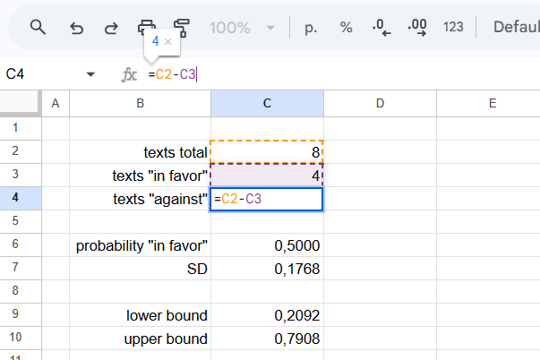
That day, 4 listeners texted in favor and 4 texted against. But no two days are the same. Today it’s one set of listeners, tomorrow it’s another, and the score could just as easily come out 3 to 5, 5 to 3, 2 to 6, or 7 to 1 — any combination is possible in principle. If we assume the audience really is evenly divided, then 4-to-4, 3-to-5 and 5-to-3 are somewhat more likely, while 8-to-0 or 1-to-7 are much less likely.

Technically, this is a binomial setup: out of 8 texts we expect 4 in favor, but we don’t know in advance how many we’ll actually get. If the probability that any given text is “for” is 50% (let’s assume exactly half the audience is in favor), then the standard error (SE, often written σ) of the observed share is:

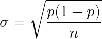
where p = 50% and n = 8.

Let’s compute it:

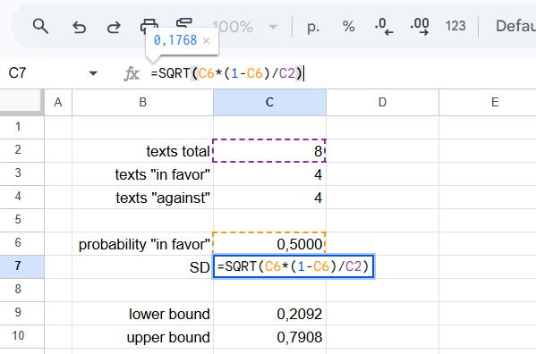
So if the probability of a “for” text is 50%, then on a sample of 8 texts the standard error comes out to 17.68%.

What does that mean in practice?

It means that because the sample (8 texts) is tiny, the amount of randomness baked into the “4 for, 4 against” result is enormous, and we cannot confidently claim a strict 50/50 split across the entire Vesti FM audience. The only thing we can state with any confidence is that the true share of “for” votes lies somewhere within an interval around 50%. And the wider we want that interval’s reliability to be, the wider the interval itself gets.

Say we want to be 90% confident in our interval — in other words, we accept being wrong 1 time in 10. Since the normal distribution is a decent approximation of the binomial once n is large enough, the interval works out to 50% ± 1.645 SE.

That’s an easy calculation in Google Sheets:

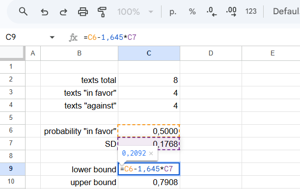
The true share of “for” votes lies in the interval 50% ± 29.08%, that is, anywhere from 20.92% to 79.08%. Roughly like this:

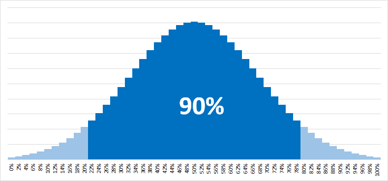
So we’re nowhere near being able to say that “listeners are splitting about 50/50.” At best — and even then we’re allowing a 10% chance of being wrong — all we can say is somewhere between 21% and 79%.

Sharpening the estimate

That said, the p ± 1.645SE interval is itself a crude approximation, and it’s at its worst exactly where we’re using it: small samples. There are more sophisticated and somewhat more accurate ways to set the bounds.

Running the numbers through the Wolfram Alpha calculator gives these bounds:

Every one of them is still enormously wide. The method you pick barely matters when the sample is this small.

So how many texts would it take to get to 45–55%?

Here’s the flip side of the question: how large would the sample have to be — still splitting exactly 50/50 — before we could narrow the interval to at least 45–55%?

That’s easy enough to solve. For an interval of 50% ± 5% (and sticking with our 90% confidence level), those 5 percentage points have to equal 1.645 standard errors. So SE = 3.04%. Plugging that back into the standard error formula:

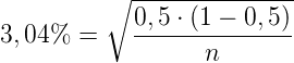
gives n = 270.6. In other words, you’d need somewhere around 271 texts, split exactly down the middle, before you could talk about a 45%–55% range at 90% confidence.

Eight texts, it turns out, is not a small sample. It’s barely a sample at all.

See also

https://en.wikipedia.org/wiki/Binomial_proportion_confidence_interval
Calculator at WolframAlpha.com
https://cyberleninka.ru/article/n/doveritelnye-intervaly-dlya-chastot-i-doley.pdf
Statistical significance for real-estate developers

In the article “Case Study: On Black Friday, KupiVIP Replaced Their Call Center with a Robot, and Only 5 Out of 5,000 People Realized They Were Talking to a Neural Network” on vc.ru, one phrase caught my attention above all else — the part where the author mentions a conversion rate increase from 6% to 8%:

Naturally, I started wondering: on what call volume was this conversion rate increase observed, and was that volume sufficient to make a reliable claim that the voice robot outperforms live call center agents?

The question can be formulated precisely as follows: what is the minimum number of calls required to claim, with a confidence level of, say, 95%, that the conversion rate “increased from 6% to 8%”?

Building the Experiment in Google Spreadsheets

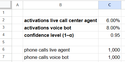
Let’s lay out the available data in Google Spreadsheets. For the calculations that follow, we’ll need a “number of calls” parameter — let’s assume for now that both the robot and live agents each made 1,000 calls before the 6% and 8% conversion rates were obtained:

Essentially, this is a standard A/B split test, and we’ll need to walk through its algorithm to obtain the Z-score and calculate the p-value.

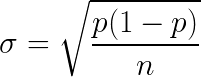
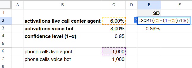
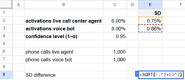
Let’s calculate the standard errors (SD, or σ) for both conversion rates, along with the standard error of the difference between them. The formula for the standard error of a conversion rate:

where p is the conversion rate (6%, for example) and n is the sample size (1,000 calls). Here’s the Google Spreadsheets calculation:

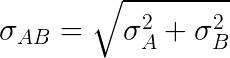
The standard error of the difference between conversion rates is calculated using the formula:

where σ is the standard error of each conversion rate, A and B (live agent and robot). We’ll compute it just below in Google Spreadsheets:

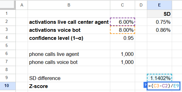
How much larger is the difference between conversions A and B compared to the standard error of that difference? This ratio is called the Z-score. In Google Spreadsheets, it’s straightforward:

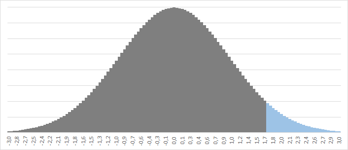
So the Z-score = 1.7541. On the normal distribution curve, this corresponds to the 96th percentile — meaning the probability of the Z-score randomly exceeding 1.7541 is about 4% (in other words, 96% of the area under the bell curve falls within +1.7541 standard deviations):

Where did we get 96%? The exact probability, the p-value, is calculated using the formula:

=NORM.DIST(1.7541,0,1,TRUE)

P-value = 96.03%.

So here’s our interim conclusion: if, on a sample of 1,000 calls in each of the two groups, we observed conversion rates (promo code activations) of 6% and 8%, then we are 96% confident that this difference is not due to chance. (There remains a 4% probability that the observed difference is random. In that case, perhaps the conversion rate is actually the same — say, 7% — and had we made more calls, the difference would have eventually disappeared.)

Minimum Experiment Size

Now, let’s get back to the original question.

We weren’t trying to prove that 8% is greater than 6%, and the figure of 1,000 calls for the robot and agents was chosen arbitrarily. What we wanted to calculate was the minimum number of calls needed to establish the statistical significance of the difference between 8% and 6% at a 95% confidence level.

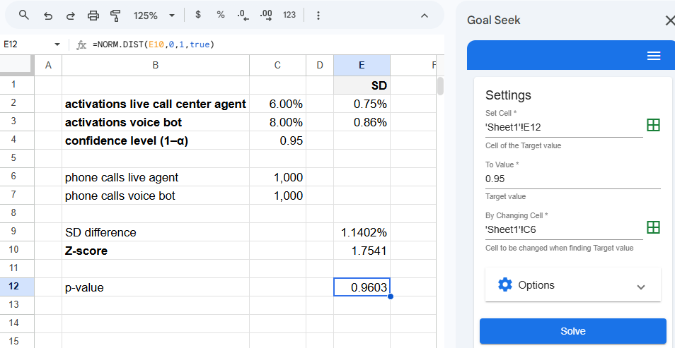
1,000 calls turned out to be more than enough. Now we just need to decrease this number until the p-value crosses the 95% threshold. (By the way, according to the normal distribution formula, this corresponds to a Z-score of 1.6449 — try verifying this yourself.)

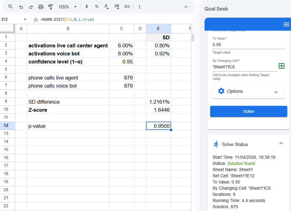
In theory, it would probably be possible to derive a large formula for the n at which the p-value equals 0.95. In practice, it’s faster to manually find the minimum n through trial and error. Or, better yet, install a Goal Seek add-on for Google Spreadsheets and use it to find the answer automatically:

(Just make sure the number of robot calls is exactly the same as the number of live agent calls, i.e., you’ve entered =C6 in cell C7.)

Conclusions

So, we’ve calculated the minimum experiment conditions for evaluating the effectiveness of the KupiVIP voice robot.

You need at least 879 calls in each of the two groups to confirm, with a 95% confidence level, that there is a difference between the 6% promo code activation rate in the control group (real live agents) and the 8% rate in the test group (voice robot).

(The only caveat is that neither 6% nor 8% yields a whole number of activations on a sample of 879 calls, and in reality, of course, the numbers would be different — and the number of calls in the two groups could vary as well. But this doesn’t really matter much, since the conversion rates cited in the article were most likely rounded.)

See also:

https://abtestguide.com/calc/?ua=1000&ub=1000&ca=60&cb=80

A contractor swears the phones drop out on every fifth call. You make one — it’s fine. Another — also fine. How many do you need before you can confidently tell him he’s wrong?

Our job is to check whether the claim that 20% of calls have connection problems holds up. And as always, we’re not going to just make 100 test calls — we don’t have the resources for that. Instead, we’ll state a null hypothesis, an alternative hypothesis, and test it at a chosen confidence level.

Stating the hypothesis and choosing a confidence level

The null hypothesis (H₀) is the contractor’s claim: at least 20% of calls have connection problems. This is the claim we’re putting on trial.

The alternative hypothesis (H₁) is that the connection is fine — problems happen in fewer than 20% of calls. This is the position we’ll lean toward if the data supports it.

(That framing matters. In hypothesis testing, you never “prove” H₀; you either reject it or you fail to reject it. So when we say we want to side with the contractor or not, what we really mean is: can we gather enough evidence to reject his claim?)

The confidence level is how sure we want to be about the outcome. The higher it is, the more test calls we’ll need to make, so we’ll budget 1% for error and go with 99% confidence — leaving a 1% chance that we reject the contractor’s claim when problems really are there.

Building the formula for the sample size

To reject H₀, all we need is to pull off N successful calls in a row with no signs of trouble — while keeping the probability at or below 1% that we simply got lucky and that real equipment problems just happened not to show up in any of the N calls.

If the contractor is right, 80% of calls go through cleanly. The probability of no issues across N calls in a row is 0.80^N. We need the smallest N for which that probability drops to 1%:
0.80^N = 0.01

Which is exactly the logarithm of 1% to base 80%.

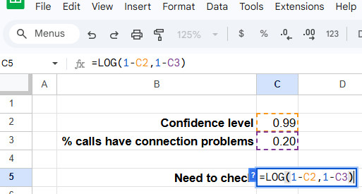
Into Google Sheets it goes:

The formula for cell C5 looks like

=LOG(1-C2,1-C3)

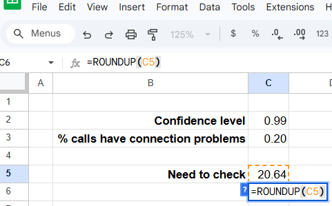
We need 20.64 calls. (Check: 0.80^20.64 = 0.9995%, right on target.)
All that’s left is rounding up:

=ROUNDUP(C5)

or, in one shot,

=ROUNDUP(LOG(1-C2,1-C3))

Testing the hypothesis

If the contractor’s claim H₀ is correct and every fifth call really does have trouble, then the probability of seeing zero problems across 21 test calls in a row is about 1%. In other words: either we just hit a one-in-a-hundred coincidence, or the claim that 20% of calls have problems doesn’t hold. At the 99% confidence level, we reject H₀ — in everyday terms, the connection is fine.