Here’s another case. The middle of a busy day in the sales department, and the phone has been silent for half an hour.

There are two possibilities: either something is broken, or this is just a lull that happened to run long, and the next customer call is about to come in.

Let’s work out how many minutes you can sit in silence before you should start to worry.

The least obvious parameter of a phone call

What parameters does a phone call in a sales department or a call center actually have? Date and time, speed of answer, duration, day of the week, line number, customer number – those are the obvious characteristics you can analyze incoming calls by.

One more hides in the shadows: the length of the pause (the stretch of time with no calls) that came right before the call. Say a call came in at 2:07 p.m. on February 13 and lasted 3 minutes 52 seconds. That’s what you see in an export, in the PBX logs, or in the CRM. What is no less interesting: if the previous call was logged at 2:01 p.m., then that six-minute gap is exactly the non-obvious parameter that could be analyzed too.

Let’s take calls to a call center on weekdays between 10 a.m. and 7 p.m. We compute the difference in minutes between two adjacent calls – “0” if less than a minute passed, “1” for one to two minutes (from 01:00 to 01:59), and so on. Analyze thousands of calls, and you get roughly this table:

(Strictly speaking, pauses longer than 40 minutes occur as well, but their share is vanishingly small – which is why, rounding to the nearest tenth, we already reach 100% at 40 minutes.)

The simple idea of “anomalous” pauses

So we now have a remarkably clean histogram of how pause lengths are distributed. What stands out is that they decay exponentially:

Let’s come back to what we set out to calculate in the first place.

The idea we started with: sooner or later, a gap between calls in the middle of the workday grows so long that it starts to worry the managers. It stands to reason that the length that triggers the worry is different in every sales department and every call center – for a large call center, a five-minute gap is already very unlikely; for another, five minutes is the standard interval between calls, but 55 minutes is genuinely suspicious.

What if we frame the idea of an “anomalously” long pause this way: it is a pause that occurs extremely rarely – say, once a week, or once a month, or once every six months. We pick the level of “anomaly” that seems reasonable to us, and then work out which pause lengths occur about as rarely as our definition says.

For example, let an anomalous pause be one that, on average, happens once a week.

If the calls in our table cover the past year, then the number of “anomalous” (“once a week”) pauses in it should be on the order of 52 – one for each week.

So we need to count off the 52 calls with the longest pauses before them. In my table there turned out to be 47 calls with pauses of 38 minutes or more, and after that 57 calls with pauses of 37 minutes or more.

Which leads to the conclusion that a 37- to 38-minute gap between calls on a weekday should put you on alert: either you are looking at the weekly “anomaly,” the one that shows up about 52 times a year, or a technical failure has occurred and the calls have stopped coming in.

Calculating Sample Size for Quality Call Audits

A common tool for assessing the quality of sales managers’ work is quality auditing of phone calls, or “call monitoring.”

Suppose your goal is not simply to measure the quality of phone calls, but to document growth in that quality. For example, you conducted training for your managers, introduced new incentives for meeting quality standards, or implemented some other intervention.

It’s reasonable to assume that an improvement in quality in the first random call recorded after the training won’t definitively prove that quality has improved across all calls. Likely, a second successful call won’t conclusively confirm the hypothesis either.

Thus, you’ll need to listen to — if not all calls — at least a sufficient number of calls after your changes, and the number of calls you’ll need to audit can, in fact, be calculated precisely.

Calculating Sample Size

On page 35 of the paper “Introduction to Statistical Inference and Experimental Design” I found a suitable example 1.9 and a formula for calculating such samples:

In this example, an improvement in ACT math test scores from 24.5 (variance 8.2) to 26.0 points is considered, with α = 0.05 and power = 0.90.

For convenience, I assembled the formula in a Google Sheet:

Sample Size Calculator

You simply need to copy the file and substitute your own values.
It’s reasonable to choose a confidence level between 80% and 95%, and a statistical power between 60% and 80%. Enter the average call quality score before changes, the standard deviation (SD) of call scores “before,” and the expected average call quality score “after” your changes.

See also:

https://bpb-us-e1.wpmucdn.com/sites.ucsc.edu/dist/2/1389/files/2026/03/part1.pdf

A curious thing about working with the concept of conversion rate is that, strictly speaking, a conversion rate is almost never precisely defined.

All those “call-to-sale conversion of 18.4%,” “CTR of 3.1%,” “deal conversion of 30%” — it’s always a somewhat simplified approach, as if the conversion rate were reliably measured and, should it change, we’d explain it with objective factors, never entertaining the thought that there never was any “18.4%” to begin with — there were just 38 contracts we closed on 206 calls, and that doesn’t at all mean there couldn’t have been more or fewer.

Much like the position of an electron around the nucleus of an atom isn’t defined by exact coordinates, but is merely described by a region where it’s most likely to be found, our conversion rate is not a specific number either. In reality, it is an interval within which it lies.

Calculating Conversion Rates and Cognitive Bias

Consider a fictional sales department that started selling a new product this year. Let’s say, hmm, trucks. The product isn’t in high demand, so, for now, there isn’t much data for analysis — or, better said, very little at all:

As the sales data shows, over several months we’ve got 4 deals out of 200 leads, i.e. our conversion rate is 4 / 200 = 2.0%.

(Additionally, based on five months of data, we can roughly project 480 leads for the next year and, accordingly, 480 × 0.02 = 9.6 deals.)

Given such scarce data, it’s impossible to go wrong, so, of course, such a forecast won’t be incorrect. However, it contains an important cognitive bias: 2.0% is not the exact value, but rather the most probable so far value of our lead-to-sale conversion rate for trucks.

In reality, the conversion rate cannot be determined precisely. It lies within a confidence interval from 0.4% to 3.6%. And for the coming year, we should be projecting not 9.6 deals, but somewhere between 5 and 15 trucks sold. Unfortunately, narrowing this range any further would be overly optimistic.

The Conversion Bell Curve

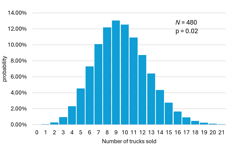
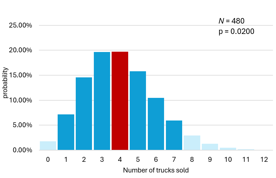
Assuming that our true conversion rate is stable and exactly equals 2.0%, we can estimate the possible range of deals out of 480 leads expected next year. Since we can only vouch for the consistency of our own work but can’t account for randomness (customer moods, force majeure, a lucky sale to the CEO’s buddy), there’s always a chance the number of deals will differ slightly from the projected 480 × 0.02 = 9.6 deals — much like the number of tails in 480 coin flips may differ slightly from 240, coming out to 235, 248, or possibly even 223.

Graphically, this looks like a normal distribution bell curve, where the further we move from the expected value of 9 deals at the center of the bell, the lower the probability of closing significantly fewer or significantly more deals:

Looking at the resulting graph, we have to admit that seeing fewer than 2 or more than 19 sales is practically impossible.

But can we narrow our confidence interval?

Confidence Interval of a Conversion Rate

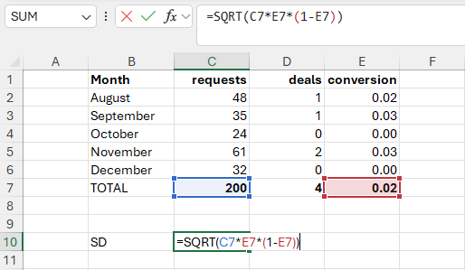
The standard error (SD) for a binomial distribution is calculated using the formula:

where n is the number of trials, and p is the probability of success.

For our 200 leads this year, we get:

SD = 1.98 deals. In other words, according to the laws of normal distribution (and binomial distribution is a special case of normal distribution), in roughly 68% of cases, while operating with a true conversion rate of 2.0%, we’d land within the confidence interval of 2.02 to 5.98 deals, i.e. ±1SD.

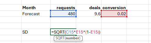
For the projected 480 leads next year, we get:

SD = 3.07 deals. By the laws of binomial (normal) distribution, it is known that in 68% of cases, next year’s sales will fall within ±1SD of the expected value of 9.6 deals, and in 90% of cases — within ±1.645SD of the expected value. 3.07 deals × 1.645 = 5.05 deals, meaning that in 90% of cases, if we work the entire next year at a 2% conversion rate, we won’t fall outside the confidence interval of “4.55 to 14.65 deals.” (Notably, conversely, in 1 out of 10 cases we will fall outside these bounds, all while still operating at a “true” conversion rate of 2%.)

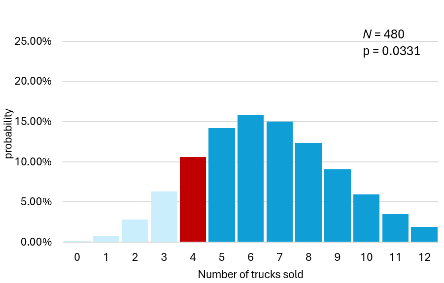
One can only wonder what kind of uproar the sales manager would raise if, by year’s end, we sold just 4 trucks on 480 leads, formally showing a conversion rate of 0.83%... and what’s even more curious is that, statistically, this happens in 1 out of 27 sales departments.

In one out of 27 cases, you get fired for missing your sales target, even though you were still operating at a “true” conversion rate of 2%.

Three Conversion Rates at the Confidence Interval Boundary

So how should we interpret this year’s results, where we got 4 sales out of 200 leads?

Case one, “2.00%.” We covered this one right away. 4 / 200 = 0.02, meaning our conversion rate is 2%. At the same time, by the laws of binomial distribution, there’s still a chance of fluctuating within the 90% confidence interval of “±1.645SD,” i.e. within the range of 0.74 to 7.26 deals per 200 leads.

It looks roughly like this:

Our result of 4 deals matched the expected value for a 2.0% conversion rate, although, in general, it didn’t have to — it could have landed anywhere within the 90% confidence interval of 1 to 7 sales.

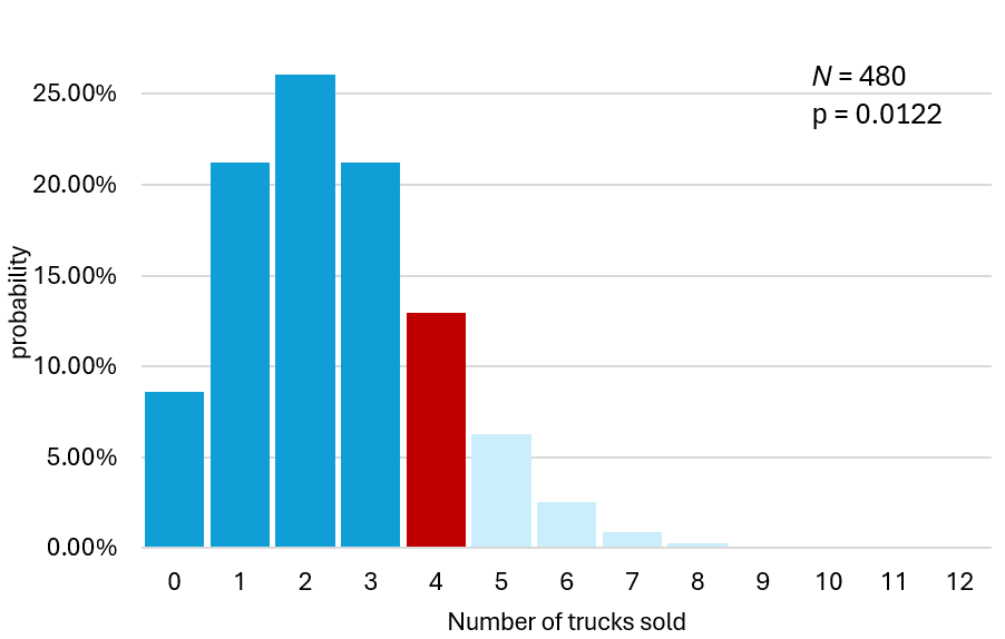
Case two, “1.22%.” In this scenario, our “true” conversion rate is actually lower, equaling, say, 1.22%. Then the expected number of trucks sold is approximately 2, and we were lucky to close 4 sales. Our luck was such that we could have made more than 4 sales only in 10% of cases. That is, we remain within the 90% probability field, though we’re sitting at its boundary. A little more, and our luck would be too good — but for now, we’re lucky “within reason”:

Case three, “3.31%.” Now let’s suppose that this year we were unlucky, even though our true conversion rate was above 2.0% all year and actually equaled 3.31%. The expected value for 200 leads would then be approximately 6 trucks sold, and making fewer than 4 sales would only be possible in 10% of cases. So we’d still be within the 90% probability field, but sitting at the left boundary with our unlucky 4 deals.

Thus, the takeaway is clear: we don’t know for sure which of the 3 conversion rates is the true one. We’re used to thinking it’s Case 1 — dividing 4 sales by 200 leads and getting a conversion rate of 2.00%. But nobody knows for certain whether the current year was typical or atypical, whether we were lucky or unlucky. In 90% of cases, it could have been a matter of luck, and we were actually operating at a conversion rate of 1.22%, or a matter of bad luck, where we were operating at a conversion rate of 3.31%. In all 3 cases, the probability of closing 4 sales out of 200 leads did not exceed the 90% threshold.

Unfortunately, we simply don’t have enough data yet to make more precise claims.

We Need More Data

A logical question to ask is — how much data do we need to accumulate before we can speak of a 2.0% conversion rate with any reliability? Let’s try gradually increasing the sample size (number of leads, and consequently, sales) until we see the 90% confidence interval converge around the 2.00% conversion rate value:

Needless to say, very few sales departments can generate more than a few tens of thousands of leads. Therefore, the truth is, setting sales targets and making promoting and firing decisions based on 1–5% conversion rates is madness — at these small numbers, math in sales simply doesn’t work.